Introduction to the Scenes API

The Scenes API provides a simple interface to search for and retrieve imagery from the Descartes Labs Catalog

The Scenes Guide, raster_data_access_with_scenes, is located in the guides sub-directory of example_notebooks. We’ll walk through this guide together to learn how to use Scenes, which is an all-purpose tool to search for and retrieve imagery from the DL Platform.

In this guide we’ll define an area of interest, or AOI, search for imagery for a specific date range, and pull down and display that imagery. We’ll also go over how to specify different types of imagery, using different bands and resolutions.

Working with Scenes

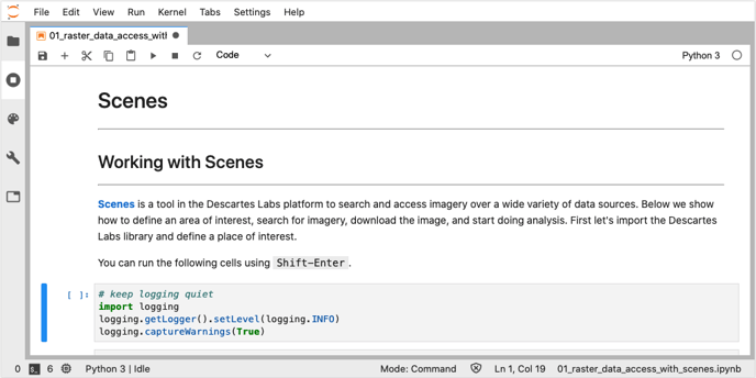
As with all Jupyter notebooks, you can run each cell by using shift & enter on your keyboard. First, we’ll import the packages needed to run this notebook, specifically the descarteslabs library.

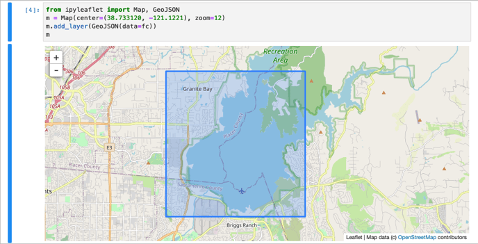
Next, we’ll define our AOI, and here, we’ll focus on Folsom Lake, a large reservoir in Northern California. To do this, we specify a GeoJSON object in this cell by defining the coordinates to create a bounding box.

Then, we can display our AOI on an interactive map, where we can zoom out, zoom in, or pan around.

Now that our AOI is defined, we can search for imagery in this region. To do so, we’ll use the scenes.search method, which will return a SceneCollection and a GeoContext. This method takes, at minimum, an AOI argument. To search for imagery from one or more products, the products argument can be used. 

Finally, limit the search results to a date range using the start_datetime and end_datetime arguments.

scenes, ctx = dl.scenes.search(
    aoi=feature,
    products='sentinel-2:L1C',
    start_datetime='2019-07-31',
    end_datetime='2019-08-05'
)

We can look at the SceneCollection to see that 2 images match our query and the dates on which those images were collected. The GeoContext tells us information about the resolution, coordinate system, and bounding box.

The scene collection can be indexed like any Python list to display more detailed information about each image in the collection. This tells us the coordinate system, date of acquisition, and all associated bands, plus their resolution and data range.

If we want to get additional information about a scenes properties, we can do so by querying the scene as though it is a Python dictionary. For example, we see the date as a datetime object:

>>> scenes[0].properties.date
datetime.datetime(2019, 8, 3, 19, 3, 59, 316807)

Up until now, we’ve only queried the metadata about images that fall within our date range and AOI. To actually download imagery, we can use the ndarray method on an individual Scene, which returns a NumPy array of the image.

First, we need to set the resolution; we will use 10 meters, which is the native resolution for Sentinel-2 visible bands. Next, we’ll define the bands we are interested in displaying (remember that the exact names can be found by looking in Catalog).

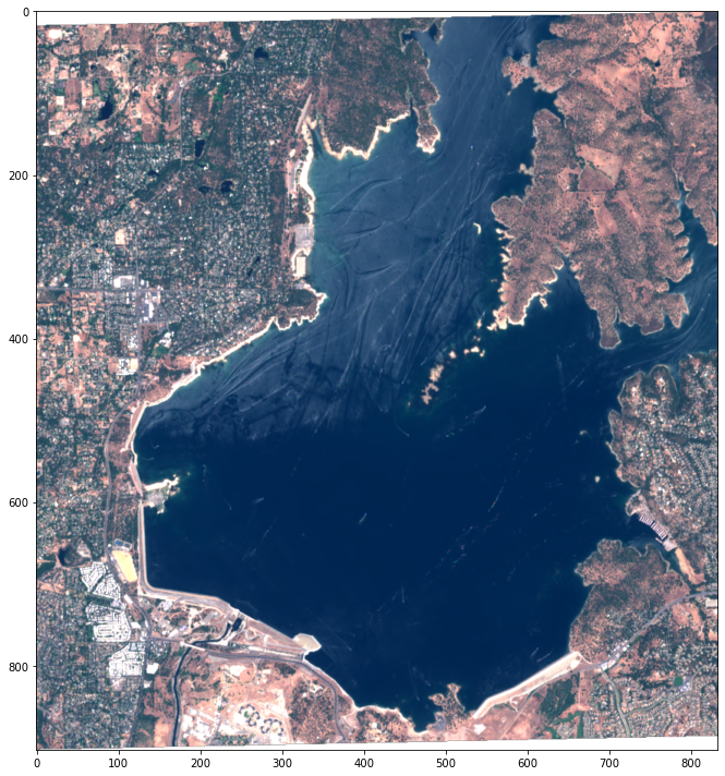
Because the image is now represented as a NumPy array, we can perform typical NumPy operations on the image. For instance, to check the shape of the image, we can use a.shape, which returns (3, 903, 833): 3 bands (red, green, blue), 903 pixels tall (y-axis), 833 pixels wide (x-axis). Because the resolution of each pixel is 10 meters, our AOI covers 9030 meters latitudinally and 8330 meters longitudinally.

Finally, we’ll display the image using dl.scenes.display. This display method uses Matplotlib under the hood, and many more custom visualizations can be created by using Matplotlib directly. Finally, we can see the imagery that matched our query and look at Folsom Lake!

Programmatic Data Access

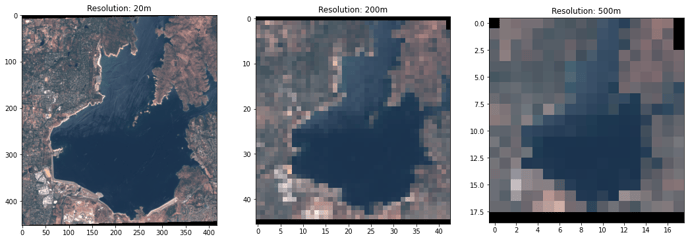
In the next section of this notebook, we look at how easy it is to manipulate our queries to view different imagery, bands, or resolutions. Scenes is powerful because it provides programmatic access to imagery, meaning we can switch our parameters with little effort.

This next piece of code allows us to specify a few different resolutions - 20, 200, or 500 meters - then display the resulting images for comparison. Imagery is resampled when ndarray is called, with the default resampling method set to nearest neighbor.

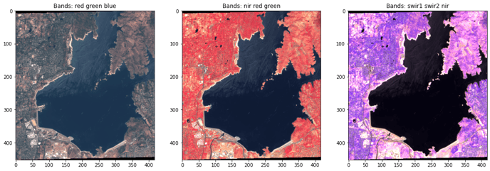
Next, we will look at bands other than visible. We can see which bands are associated with the image by looking at the properties or by looking in the Catalog. By simply setting different band names in the ndarray call, we can compare different spectra for the AOI.

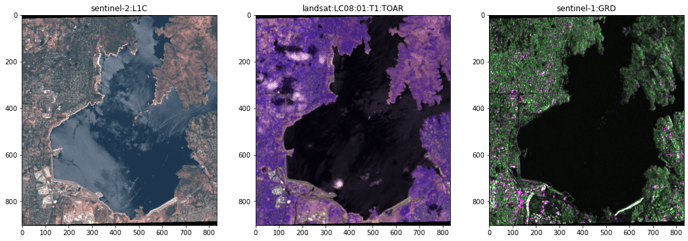
Finally, we can look at imagery from different sources over the same AOI. This is a simple definition, this time in the search method, and we can easily display and compare different types of imagery.

This is just a quick overview of Scenes functionality. As always, please consult our resources to dig deeper. And check out our other videos to learn more about Descartes Labs tools!